The Perceptron Learning Algorithm (PLA) is one of the simplest Machine Learning (ML) algorithms. This post goes through an elementary example to illustrate how PLA works.

Notes on Perceptron Learning Algorithm

We start with some definitions and classification problem outline, next we move to the plain vanilla perceptron learning algorithm.

Linear Classifier

Consider set of points $X=\{x_i \in R^{n+1}, i=1, \dots ,N\}$ with first coordinate fixed to 1 and mapping $X \to Y$ where $Y=\{-1,1\}$ , which maps elements of $X$ to two different classes denoted by elements of $Y$ . The two classes are assumed to be linearly separable, i.e. there exists vector $W \in R^{n+1}$ such that $Y(x) = sign(W * x)$ where * is dot product on $R^{n+1}$ . For the sake of the following discussion we will define $sign(0) = 1$ . Such mapping $Y$ is a linear classifier (on the set $X$ ). The set of the pairs

$T=\{ (x_i, y_i)$ : $y_i=Y(x_i), x_i \in X, i=1, \dots ,N\}$

is called the training data set.

Perceptron Learning Algorithm (PLA)

Given a training data set $T$ , the goal of PLA is to find some $W$ that provides correct classification on $T$ , i.e. for all pairs in the training set holds $Y(x_i) = sign(W * x_i) = y_i$ . Obviously, for a linearly separable training data sets such classifier is not unique.

The algorithm is iterative. On each iteration we will obtain new candidate value for $W$ , which we will denote as $w_k$ and the corresponding linear mapping will be denoted as $Y_k(x)=w_k * x$ .

Initialization. Assign $w_0 = 0$ .

Step $k$ .

Compute values of $Y_k(x_i)$ pairs on the training set until we find a misclassified pair, say, for $i$ , $Y_k(x_i) \neq y_i$ .
Update the candidate using the rule: $w_{k+1} = w_k + y_ix_i$ .

Termination. Stop iterations when all points are correctly classified.

The intuition behind the update method (item 2) is that it adjusts $w(k)$ to improve its performance on the selected misclassified point:

$Y_{k+1}(x_i) = w_{k+1} * x_i$

$= (w_k + y_ix_i)*x_i$

$= Y_k(x_i) + y_i|x_i|^2$

and since always $|x_i|^2 > 0$ , due to the first non-zero coordinate, the value of $Y_{k+1}(x_i)$ is closer to having the same sign as $y_i$ than $Y_{k}(x_i)$ . Since each step improves only on a single training pair (and may actually make classification performance worse on some or all other pairs), it is not obvious why the PLA converges to a solution of the linear classification problem. The proof will be discussed in one of the future posts. Here we will use an extremely simple examples to illustrate the PLA.

Example: One-dimensional Training Data Set.

The training data set consists of two training points:

$x_1 = (1,2), y_1 = -1$ ;

$x_2 = (1,-0.25), y_2 = 1$

also shown below:

Figure 1. Training set. First coordinate of x is not shown (=1).

While this is probably the simplest example that can be devised to illustrate the PLA, it shows the idea behind it in a clear unobstructed way. By executing the PLA step-by-step we will first initialize $w_0 = (0,0)$ .

Iteration 1. We obtain:

$Y_0(x_1) = sign(w_0 * x_1) = sign(0 * 1 + 0 * 2) = sign(0) = 1$ ;

$Y_0(x_2) = sign(w_0 * x_2) = sign(0 * 1 + 0 * ( - 0.25)) = sign(0) = 1$ .

Note that $Y_0$ classifies the entire range of real values of $x$ as +1. Out of the two training data points only the first one $x_1$ is misclassified: the desired value is -1 while $Y_0(x_1)$ returns +1. This results in an update:

$w_1 = w_0 + (-1)*(1, 2) = (-1, -2)$

Iteration 2. With the new candidate $Y_1(x)=w_1*x$ we obtain the following values on the data points:

$Y_1(x_1) = sign(w_0 * x_1) = sign( ( - 1) * 1 + ( - 2) * 2) = sign(-5) = -1$ ;

$Y_1(x_2) = sign(w_0 * x_2) = sign( ( - 1) * 1 + ( - 2) * ( - 0.25)) = sign(-0.5) = - 1$ .

As a side note, the decision boundary between the two classes is now located at $x = -0.5$ (while for $Y_0$ it was at -∞):

Figure 2. Decision boundary after first iteration.

The value $x = -0.5$ of decision boundary is obtained by solving equation:

$w_0 * x = 0$ or, equivalently, $(-1) * 1 + ( - 2) * x = 0$ .

The misclassified point $x_2 = (1, - 0.25)$ leads to an update:

$w_2 = w_1 + 1*(1, -0.25) = (0, -2.25)$

That moves decision boundary to the root of the equation $0 * 1 + x * (-2.25) = 0$ i.e. to $x = 0$ and results in all training data points classified correctly:

Figure 3. Second iteration moves decision boundary to classify all points correctly.

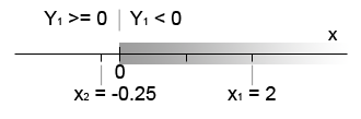
Figure 3. Second iteration moves decision boundary to x=0. Both training data points are classified correctly.

References

The PLA is covered by many books and articles. The AML Book listed below is easily accessible, well written and has a corresponding MOOC.

[1] Yaser S. Abu-Mostafa, Malik Magdon-Ismail, Hsuan-Tien Lin. “Learning From Data” AMLBook, 213 pages, 2012.

3DMatics

Notes on Perceptron. Part 1: The Perceptron Learning Algorithm.

Notes on Perceptron Learning Algorithm

Linear Classifier

Perceptron Learning Algorithm (PLA)

Example: One-dimensional Training Data Set.

References

Find

Content

Home

Archives

RSS Feeds

3DMatics

Notes on Perceptron. Part 1: The Perceptron Learning Algorithm.

Notes on Perceptron Learning Algorithm

Linear Classifier

Perceptron Learning Algorithm (PLA)

Example: One-dimensional Training Data Set.

References

Find

Content

Home

Tags

Archives

RSS Feeds