Generating artificial test data for Machine Learning (ML) algorithms is an important step in their development. This post discusses generation and plotting of linearly separable test data for binary classifiers like Perceptron.
Artificial Linearly Separable Test Data in Python
We start with defining linear function on n-dimensional space and the binary classifier associated with it. Next we move to generating artificial test data and plotting it.
Test Linear Classifier
In anticipation of using it for Perceptron Learning Algorithm (PLA) tests we add another dimension for vectors to hold the class of the training sample. The training data structure is a numpy array with first column all set to 1 and the last column holding class assignment, meaning 2D data results in allocating and holding 2-dimensinoal array 4 x n_points.
'''
Module linear_func.py
************************

Defines a linear function and a linear classifier
based on the function.
'''
import numpy as np

class Classifier:
    '''Class to represent a linear function and associated linear
    classifier on n-dimension space.'''

    def __init__(self, vect_w=None):
        '''Initializes coefficients, if None then
        must be initialized later.

        :param vect_w: vector of coefficients.'''
        self.vect_w = vect_w

    def init_random_last0(self, dimension, seed=None):
        '''
        Initializes to random vector with last coordinate=0,
        uses seed if provided.

        :params dimension: vector dimension;

        :params seed: random seed.
        '''
        if seed is not None:
            np.random.seed(seed)
        self.vect_w = -1 + 2*np.random.rand(dimension)
        self.vect_w[-1] = 0  # exclude class coordinate

    def value_on(self, vect_x):
        '''Computes value of the function on vector vect_x.

        :param vect_x: the argument of the linear function.'''
        return sum(p * q for p, q in zip(self.vect_w, vect_x))

    def class_of(self, vect_x):
        '''Computes a class, one of the values {-1, 1} on vector vect_x.

        :param vect_x: the argument of the linear function.'''
        return 1 if self.value_on(vect_x) >= 0 else -1
As a side note, we could define both linear function and the associated classifier using closures and lambda, but that would leave the coefficients of the function not directly accessible (we would need to compute them unless we specify them explicitly). Also it would make it less convenient adding more functionality like the utility for plotting we are discussing next.
Let’s add to Classifier class a utility function to simplify 2D plotting. The purpose of this function is to return a pair of points used to draw the decision boundary within specified box (axis-aligned rectangle). The decision boundary is the line where the value of the function equals 0. An important note is that for simplicity we skip checks for special cases when the line is parallel to one of the axis. We may generalize (later) the function by passing in selection of two coordinates to handle the case the classifier is defined in higher dimension.
    def intersect_aabox2d(self, box=None):
        '''Returns two points intersection (if any) of the
        decision line (function value = 0) with axis-aligned
        rectangle.'''
        if box is None:
            box = ((-1,-1),(1,1))

        minx = min(box[0][0], box[1][0])
        maxx = max(box[0][0], box[1][0])
        miny = min(box[0][1], box[1][1])
        maxy = max(box[0][1], box[1][1])

        intsect_x = []
        intsect_y = []

        for side_x in (minx, maxx):
            ya = -(self.vect_w[0] + self.vect_w[1] * side_x)/self.vect_w[2]
            if if ya >= miny and ya <= maxy:
                intsect_x.append(side_x)
                intsect_y.append(ya)
        for side_y in (miny, maxy):
            xb = -(self.vect_w[0] + self.vect_w[2] * side_y)/self.vect_w[1]
            if if xb <= maxx and xb >= minx:
                intsect_x.append(xb)
                intsect_y.append(side_y)
        return intsect_x, intsect_y
Random Data Generator
In a separate module (let’s call it test_data_gen.py) we define generator of test data. Also we add a simplest possible test code to plot the data and the decision boundary. Having that plot gives some reassurance that the code we are going to use is at least reasonably correct. To follow the best practices we would also need to add tests to the module and make sure that special cases are handled properly. We skip all this in the current discussion to get to the action (PLA tests in the upcoming posts) asap.
import numpy as np

def separable_2d(seed, n_points, classifier):
    '''Generates n_points which are separable via
    passed in classifier in 2d.

    :params seed: sets random seed for the random
        generator,

    :params n_points: number of points to generate,

    :params classifier: a function returning
        either +1 or -1 for each point in 2d.'''
    np.random.seed(seed)

    dim_x = 2
    data_dim = dim_x + 1 + 1  # leading 1 and class value
    data = np.ones(data_dim * n_points).reshape(n_points, data_dim)

    # fill in random values
    data[:, 1] = -1 + 2*np.random.rand(n_points)
    data[:, 2] = -1 + 2*np.random.rand(n_points)

    # TODO: use numpy way of applying a function to rows.
    for idx in range(n_points):
        data[idx,-1] = classifier.class_of(data[idx])

    return data
The code above generates uniformly distributed in a box ((-1,-1),(1,1)). Of course, the box can be made a parameter but we don’t bother with this generalization. We may consider it later when we will investigate the influence of data normalization on the convergence speed of learning algorithms, in particular PLA.
The simplest possible test code with plotting the data and decision boundary is also straightforward. It uses pylab module for plotting.
if __name__ == "__main__":
    # Import * is not the best practice, but...
    from pylab import *
    import linear_classifier

    data_dim = 2
    classifier = linear_classifier.Classifier()
    classifier.init_random_last0(data_dim + 2, 130216)

    data = separable_2d(263247, 12, classifier)

    condition = data[:, 3] >= 0
    positive = np.compress(condition, data, axis=0)

    neg_condition = data[:, 3] < 0
    negative = np.compress(neg_condition, data, axis=0)

    x_pos = positive[:, 1]
    y_pos = positive[:, 2]

    x_neg = negative[:, 1]
    y_neg = negative[:, 2]

    plot_lim = 1.2
    box = ((-plot_lim, -plot_lim),(plot_lim, plot_lim))
    decision_x, decision_y = classifier.intersect_aabox2d(box)

    figure()

    ylim([-plot_lim, plot_lim])
    xlim([-plot_lim, plot_lim])

    plot(x_pos, y_pos, 'g+', label="Class=+1")
    plot(x_neg, y_neg, 'r.', label="Class=-1")
    plot(decision_x, decision_y, 'b-', label="Decision Boundary")

    plt.legend(bbox_to_anchor=(0., 0.9, 1., .102), ncol=3, mode="expand", borderaxespad=0.)

    xlabel('x')
    ylabel('y')
    title('Artificial Training Data')

    show()
It draws the following image:
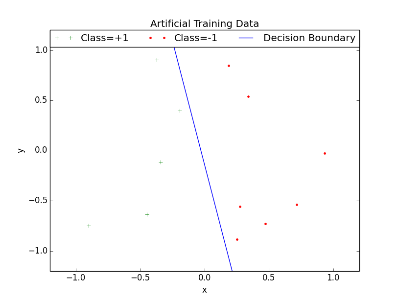
The generated data is a numpy array:
[[ 1.         -0.1928764   0.39962001  1.        ]
 [ 1.          0.25038266 -0.88412106 -1.        ]
 [ 1.         -0.89879402 -0.75034091  1.        ]
 [ 1.         -0.44705782 -0.63754637  1.        ]
 [ 1.          0.18564908  0.84809286 -1.        ]
 [ 1.          0.47149923 -0.72909877 -1.        ]
 [ 1.         -0.33891335 -0.11343507  1.        ]
 [ 1.          0.27546945 -0.55661253 -1.        ]
 [ 1.          0.93156523 -0.02588478 -1.        ]
 [ 1.          0.71528106 -0.53893679 -1.        ]
 [ 1.         -0.37236843  0.90336908  1.        ]
 [ 1.          0.34107903  0.54026163 -1.        ]]
We do not bother to add References section to this post as all of the techniques and methods are widely used, explained and can be searched for on the Internet. That makes the post to be a nearly-trivial tutorial (with some minor todos left as an exercise). In the next installment we will investigate the behavior of Perceptron Learning Algorithm (PLA) on artificial training data generated using the code form this post.

