3DMatics

This post illustrates that practical convergence for separable data of PLA is achieved much faster than the theoretical estimate suggests

Experiment vs. Theoretical Estimate

Consider a separable data set generated using methods from this post. The data set has the following values of the parameters included in formula (12) for max steps until convergence for PLA from this post:

,
,
.

Here is the max squared norm of training vectors (that are generated in the square -1,+1 resulting in value 2 plus bias 1); is norm of classifier decision vector and is margin, i.e. minimal separation of data points from decision boundary. The max number of epochs until PLA converges is estimated then as .

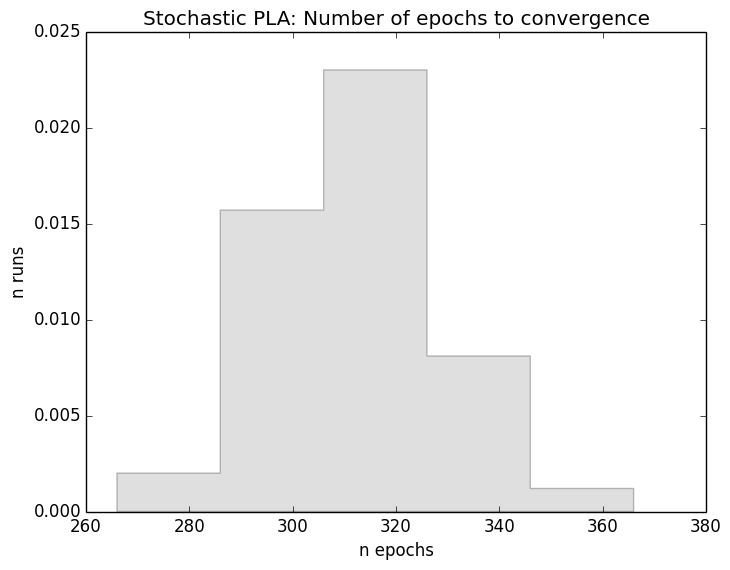
By fixing dataset with described parameters and running stochastic PLA 500 times with different random seed we obtained the following histogram of number of epochs until convergence. As the histogram shows, the theoretical estimate is higher than typical practical values by orders of magnitude. The obtained distribution is uni-modal and is centered around  value which is almost three orders of magnitude closer to zero.

The code snippet used to generate histogram is straightforward:

    epochs = []
    n_runs = 500
    for _ in range(n_runs):
        pla_rand = perceptron.PLARandomized(training_data)
        while pla_rand.next_epoch():
            pass
        epochs.append(pla_rand.epoch_id)

    n, bins, patches = plt.hist(epochs, 5, normed=1, histtype='stepfilled')
    plt.setp(patches, 'facecolor', 'grey', 'alpha', 0.25)
    plt.xlabel('n epochs')
    plt.ylabel('n runs')
    plt.title(r'Stochastic PLA: Number of epochs to convergence')
    plt.savefig("stochastic_PLA_convergence_" + str(data_dim).zfill(3) + "_" + str(n_points)+'_' + str(n_runs) + ".png",
            bbox_inches='tight')

We omitted the required import statements for brevity. Also we normalized number of runs (normed=1 in histogram parameters). The implementation of PLARandomized is essentially the same as for basic deterministic PLA with the only difference – random choice of mis-classified sample on each epoch.

References

[1] S.Haykin “Neural Networks: A Comprehensive Foundation”, 19989, Prentice-Hall, 842 pages.
[2] Yaser S. Abu-Mostafa, Malik Magdon-Ismail, Hsuan-Tien Lin. “Learning From Data”  AMLBook, 213 pages, 2012.